The Anatomy of Arrow

Arrow is an important in-memory format for analytics. Let’s go through its internals to understand why it is so appealing.

Apache Arrow is an in-memory (i.e. RAM, not disk) columnar data format. Contrarily to e.g. Apache Parquet, that is optimized for storage, Arrow is optimized for compute. If you are coming from Python, you can think of Arrow as an alternative to numpy: store values in arrays / columns to perform fast computations.

As a format optimized for compute, Arrow fulfills 3 requirements:

• any element of an array may be null
• access to any element of an array must be fast
• operations over multiple values must be fast

The goal of this post is to go through each of the items and show how Arrow fulfills these requirements. It is the in-memory format used by many query engines out there, such as Dremio, influx IOx, parts of the delta-lake, DataFusion, DataFuse, signavio, and Polars, which currently ranks as the most performant DataFrame API in the H2O benchmarks (e.g. faster than Dask, ClickHouse and Pandas).

At Munin Data, we use Arrow for all our data transformations and always recommend it for data operations where data integrity is a requirement (e.g. GxP), due to how it easily allow to preserve types, nulls and metadata, without jeopardising performance.

Null values

Anyone working with data knows that nulls in data are just a fact of life: the sensor failed, someone did not report a field in the form, and left joins are just some of the examples that lead to null values in data.

If you have used numpy or Pandas (Python), you have probably noticed that support for null values is limited: for example, Pandas does not accept a column of integers with nulls, and will cast them to floats, using “NaN” to represent null values. Engines like Spark do natively support null values, however, such support usually comes at the high cost of performance of in-memory operations.

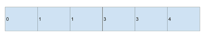
Arrow supports nulls without loss of performance in non-null values. Arrow’s design is that values and “validity” (whether a value is valid or null) are stored in two separate memory regions. To illustrate this, we are going to represent how data is stored in memory under the Arrow specification. For this, let’s consider the following array of 5 elements:

An array of 5 elements, unsigned integers (e.g. int32, 4 bytes each), whose one of the elements is null.

There are many ways to represent this in memory, with or without compression, do not store nulls, etc. In Arrow, this array is stored as two different memory regions: the values region,

The values region of a int32 array are all stored; the second element could be any number. Each element occupies 4 bytes (and are stored one after the other in the machine’s native endianness).

and validity,

Each element of the array gets a bit, and the validity is represented as bytes. The last bit is the first element, the second to last the second, etc. I.e. the first element is valid (1), the second is null (0), the 3rd–5th are valid (1,1,1). The remaining 3 bits are ignored. Larger arrays are stored with more bytes, using an equivalent counting.

The first observation is that values are stored irrespectively of whether they are valid or not. This may seem a waste of memory, but, as we will see below, it is crucial for the other two requirements.

The second observation is that validity is not stored as booleans, but as single bits. There are two main reasons for this choice: the first reason is that we gain a 8x compression factor. The second reason is performance, as we will explore in the 3rd section.

Finally, in Arrow, the validity is always optional: when an array has no nulls, we do not use (nor allocate) a validity altogether, and just operate on the values.

Fast random access

Random access in this context is the access pattern whereby an element of an array is accessed at random. Fast in this context means that accessing an element of the array (at random) must not depend on the size of the array, i.e. we must be fast at retrieving any element.

Getting the element “i” from the example array above is quite fast: go to the beginning of the values region and jump by i*4 bytes. With a small variation we do the same for the validity. This is possible because we store both nulls and non-null values; if we had not, the access would require to “count the number of valids up to i” followed by “jump by that number times 4”. This is no longer fast because the lengthier the array, the more it takes to compute the number of valid values and thus to access an element. This shows why it is important to store all values (nulls or not): it allows fast random access.

But what about the typical problem of accessing elements in string arrays, where each element has a different size, you may ask? For this, we need to learn how Arrow stores variable-sized arrays. Let’s thus consider a new example:

An array of strings. The second entry is null, the 4th entry is empty (and not null). The size of each element is not constant, so we can’t “jump by i * bytes”.

Variable-sized arrays are represented in Arrow in 3 memory regions: values, offsets, and validity. Let’s go through them to understand how they enable fast random access. The first memory region contains the bytes corresponding to the data itself:

The values are written one after the other in bytes, where nulls and empty values are not written in this region. A character may occupy more than a single byte (utf-8), which is a natural part of this representation.

The second region contains “offsets”:

The offsets are the cumulative size of the values throughout the array, plus a zero at the left most position. The the first position, the length is 1 (a), at position 1 the length continues to be 1 (“a”+””), at position 2 the length is 3 (“a”+””+”ab”), and so on.

The third region is the validity, as before:

All validity regions are represented in the same way in Arrow.

With this construction, we access the element at position “i” (e.g. i=2) as follows:

1. get the offset at positions “start=i” (offset = 1) and “end=i+1” (i+1=3, offset = 3).
2. return the slice from the values region between start and end (ab).

Like before, this is independent of the number of elements of the array, fulfilling our goal of fast random access.

Arrow supports much more complex array types, such as list arrays (an array whose elements are themselves arrays), Struct arrays (like a list of Python dictionaries), Union arrays, etc. They address further requirements for representing data. They all fulfill fast random access.

Fast compute

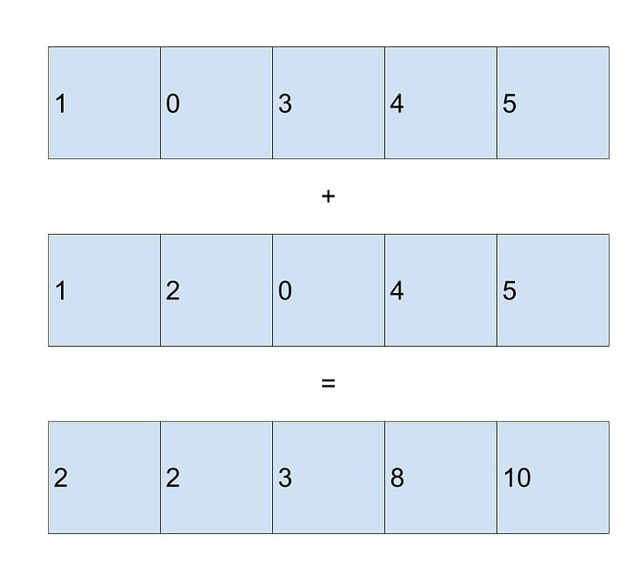
The in-memory representation of Arrow makes it very suitable for numeric operations. Let’s consider the operation of adding two integer arrays together, taking into account that if any of the values is null, the resulting value should also be null, i.e.

The usual semantics of a vertical operation with nulls: nulls remain nulls, everything else is added item by item.

A naive approach to execute this operation is to perform a for loop over both indices e.g. via “zip”, and use an if else inside the loop using the validity of each array. However, Arrow is particularly well designed for unconditional operations, which are much faster in modern CPUs.

The idea is to divide this operation in two: the first operation is to add two arrays of numbers unconditionally,

Operating over arrays of values item by item unconditionally is one of the fastest numerical operations in a modern CPU.

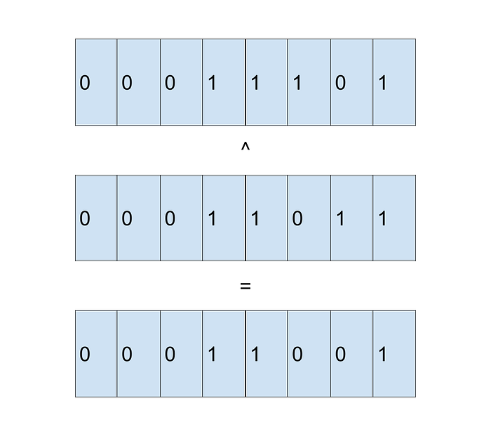
The second operation is a bitwise AND between the two validities, i.e.

Performing a bitwise AND over slices bytes is extremely efficient in modern CPUs.

Both operations benefit from using Single Instruction Multiple Data (SIMD), something that most compilers will insert in these unconditional loops. By dividing the operation in two, we (implicitly or explicitly) instruct the compiler to issue SIMD instructions, since they both fall in the category of “there are SIMD instructions for this operation in modern CPUs”. The benefits from not having to branch `if is_valid` in the loop very often outweigh (by multiples of 10) the cost. Horizontal operations such as summing all non-null elements of an array benefit equally from this format.

Summary

Choosing an in-memory format is one of the most important decisions that compute engines must take due to its groundbreaking consequences to how data is loaded, operated on, and unloaded. In this post I tried to illustrate the simplicity and strength of the Arrow format from this point of view. There are other important aspects of the Arrow format that are not mentioned in this post such as its interoperability across programming languages, which you can find more about at https://arrow.apache.org/.